
8. LSTM and GRU
A plain recurrent network struggles to carry information across many time steps because repeated multiplication by the same weight matrix makes gradients vanish or explode. Gated recurrent cells fix this by adding a state that flows through time with mostly additive updates, controlled by learned gates. This module builds the long short-term memory (LSTM) cell and the lighter gated recurrent unit (GRU), and contrasts when to reach for each.
8.1 The gating idea
A vanilla recurrent layer updates its hidden state by \(h_t = g(W_h h_{t-1} + W_x x_t + b)\). Backpropagating the loss through \(T\) steps multiplies many Jacobians of this map together, so the gradient magnitude scales roughly like the \(T\)-th power of the recurrent weight's spectral radius. Below one it vanishes, above one it explodes, and in both cases the network cannot learn dependencies that span many steps.
The gating idea introduces a separate cell state \(c_t\) that is updated mainly by addition rather than by a full matrix multiply. When the update leaves the previous cell state untouched, the gradient of \(c_t\) with respect to \(c_{t-1}\) is close to the identity, so error signals flow backwards over long spans without shrinking. This near-identity path is the constant error carousel.
Remark: the key word is additive. Multiplicative recurrence compounds a factor at every step, while an additive path lets the state persist by default and change only when a gate opens.
8.2 The LSTM cell
Throughout, \([h_{t-1}, x_t]\) denotes the concatenation of the previous hidden state and the current input into one vector. Each gate is a vector in \((0, 1)\) produced by a sigmoid \(\sigma\) applied to an affine map of that concatenation, so a gate value near \(1\) lets information through and a value near \(0\) blocks it.
8.2.1 The three gates
The forget gate \(f_t\) decides how much of the old cell state to keep, the input gate \(i_t\) decides how much of the new candidate to write, and the output gate \(o_t\) decides how much of the cell state to expose as the hidden state:
\[\boxed{ f_t = \sigma\!\left(W_f\,[h_{t-1}, x_t] + b_f\right), \quad i_t = \sigma\!\left(W_i\,[h_{t-1}, x_t] + b_i\right), \quad o_t = \sigma\!\left(W_o\,[h_{t-1}, x_t] + b_o\right) }\]Remark: the gates share the same functional form and differ only in their learned parameters. The bias is explicit here, exactly as with the feedforward layers of earlier modules, and is never folded into the weight matrix.
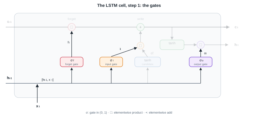
The cell so far: three sigmoid gates reading \([h_{t-1}, x_t]\) from the input rail. The paths they will control are still grayed out.
8.2.2 Candidate and cell update
A \(\tanh\) layer proposes a candidate update \(\tilde{c}_t\), the new content the cell could store:
\[\boxed{ \tilde{c}_t = \tanh\!\left(W_c\,[h_{t-1}, x_t] + b_c\right) }\]The cell state is then updated by keeping a gated fraction of the past and adding a gated fraction of the candidate, with \(\odot\) the elementwise (Hadamard) product:
\[\boxed{ c_t = f_t \odot c_{t-1} + i_t \odot \tilde{c}_t }\]When \(f_t \approx 1\) and \(i_t \approx 0\) the cell simply copies \(c_{t-1}\), which is the constant error carousel: \(\partial c_t / \partial c_{t-1} \approx \mathrm{diag}(f_t)\), so gradients pass through nearly unattenuated.
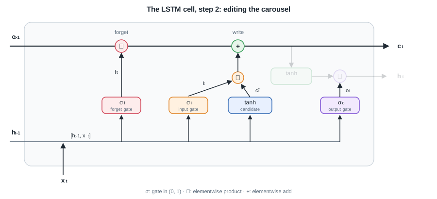
Step 2 lights up the carousel: the candidate proposes content, the forget multiply and the write add edit the cell state as it crosses the top. Only the output side remains gray.
8.2.3 Hidden state
The hidden state is the squashed cell state, gated by the output gate:
\[\boxed{ h_t = o_t \odot \tanh(c_t) }\]Remark: the cell state \(c_t\) is the long-term memory that flows along the carousel, while the hidden state \(h_t\) is the filtered view exposed to the next layer and to the output at this step. Keeping them separate is what distinguishes the LSTM from the GRU below.
The whole cell, assembled:
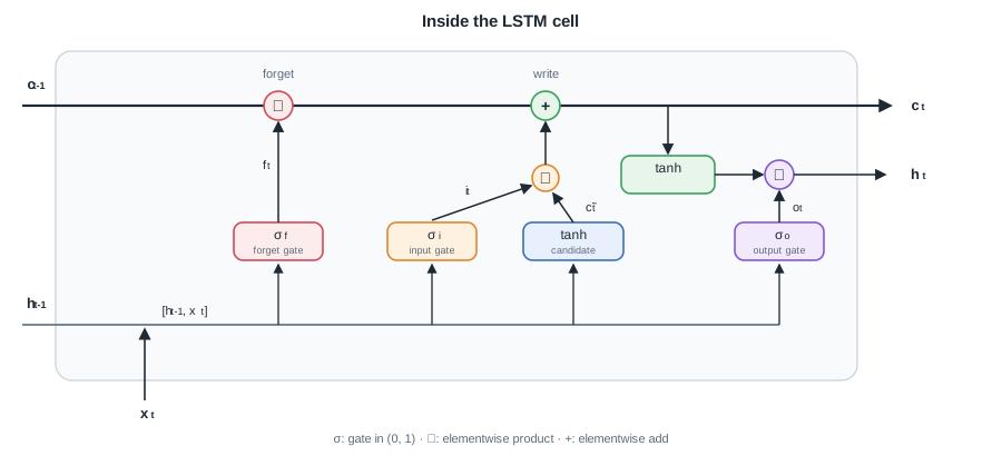
One LSTM step. Along the top runs the carousel: the cell state crosses the cell touched only by the forget multiply and the write add, never by a matrix multiply. Below, the four blocks read \([h_{t-1}, x_t]\) and decide what to forget (\(f_t\)), what to write (\(i_t \odot \tilde{c}_t\)), and what to expose (\(h_t = o_t \odot \tanh(c_t)\)).
8.3 The GRU
The GRU merges the cell and hidden state into a single \(h_t\) and uses only two gates, so it has fewer parameters while keeping the additive-update benefit.
8.3.1 Reset and update gates
The reset gate \(r_t\) controls how much past state feeds the candidate, and the update gate \(z_t\) controls how much of the state to refresh:
\[\boxed{ r_t = \sigma\!\left(W_r\,[h_{t-1}, x_t] + b_r\right), \quad z_t = \sigma\!\left(W_z\,[h_{t-1}, x_t] + b_z\right) }\]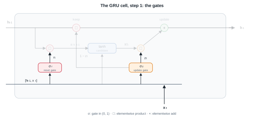
The cell so far: just two gates on the input rail, the state path still grayed out.
8.3.2 Candidate and interpolated state
The candidate uses a reset-gated version of the previous hidden state, and the new state is a gated interpolation between the old state and the candidate:
\[\boxed{ \tilde{h}_t = \tanh\!\left(W\,[\,r_t \odot h_{t-1}, \; x_t\,]\right), \quad h_t = (1 - z_t) \odot h_{t-1} + z_t \odot \tilde{h}_t }\]Remark: the interpolation form ties the keep and write fractions together with a single gate: whatever weight \(z_t\) gives the candidate, \(1 - z_t\) is left for the past. The LSTM sets its keep fraction \(f_t\) and write fraction \(i_t\) independently, which is one more gate and one more matrix.
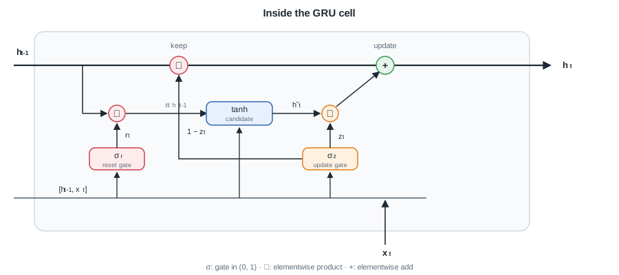
One GRU step. The reset gate \(r_t\) filters how much of the past feeds the candidate, then the update gate splits the state between keeping (\(1 - z_t\)) and refreshing (\(z_t\)). One state line, two gates, same additive path.
8.4 LSTM versus GRU
Both cells solve the vanishing-gradient problem with an additive state path. They differ in how many gates carry that path and whether the long-term memory is kept separate from the exposed state.
| Aspect | LSTM | GRU |
|---|---|---|
| Gates | 3 (forget, input, output) | 2 (reset, update) |
| Separate cell state | yes (\(c_t\) and \(h_t\)) | no (single \(h_t\)) |
| Parameters per unit | more (four affine maps) | fewer (three affine maps) |
| Keep and write | independent (\(f_t\), \(i_t\)) | tied (\(z_t\) and \(1 - z_t\)) |
| Prefer when | long dependencies, ample data and compute | smaller data, faster training, similar accuracy |
Remark: in practice the two often reach comparable accuracy. The GRU trains faster and generalizes well on smaller datasets, while the extra capacity of the LSTM can help on very long sequences. Treat the choice as a tunable hyperparameter rather than a settled rule.
Gates let a recurrent state persist over long spans, but they still read one step at a time. The next part lets every position attend directly to every other, removing the sequential bottleneck.
Next: Attention · Course overview